Youth hockey stats template excel spreadsheet

By Dave MacPherson | Posted Aug 19, 2020

In July 2019, I launched Pick224, a hockey analytics website containing data from over 15 hockey leagues across the world with a focus on junior hockey and the NHL draft. To compile this data, I first scrape all the individual game summaries of each league, then clean the data, total up all the stats, and join the results with each player’s biographical information.

Since launching, I’ve written blogs on how to scrape hockey data, whether from HTML web pages or sites that use JSON. I’ve since gotten a lot of questions from scouts and others who work in hockey asking about the next steps: cleaning and summarizing data.

If you have some experience with Excel or Google Sheets and don't want to start learning a programming language like R or Python, but still want to get shit done, this post is for you. Excel and Google Sheets are powerful tools, and it’s okay if you’re not ready to learn a programming language. After you get a good understanding of the things you can do with data, you can then decide if you would like to do those things more efficiently and effectively using R or Python. You may also want to start with R or Python if you're working on a project with more data than Google Sheets or Excel can handle.

In the following sections, I’ll walk through the whole process of turning raw hockey data into the summarized player totals you see on Pick224, all using Google Sheets. When I first launched Pick224, my database was entirely built using the methods below.

I recommend following along and working through the formulas. Here’s a file containing only the raw data that you can make a copy of and follow along with, and here’s a copy of a final file, after having worked through everything below.

The raw data

To prepare for this write-up, I wrote some scrapers to pull everything I needed from the Czech U20 league’s 2020 season. This data includes:

• A schedule of all games, containing a unique identifier for each game
  • Fields: GAME_ID, HOME_TEAM, AWAY_TEAM
  • Fields: GAME_ID, H_A (Home or Away team), J_NO (jersey number), POS (position), NAME, PLAYER_URL
  • Fields: GAME_ID, GOAL_ID, TEAM, SCORER, ASSISTS, STR (goal strength), PLAYER_URLS
  • Fields: GAME_ID, GOAL_ID, PLUS_OR_MINUS, PLAYER_IDS

  The goal

  Using all of this raw data, we will be calculating the following season stats for each player who played at least one game:

  • GP - games played
  • EV_G - even-strength goals
  • EV_A1 - even-strength primary assists
  • EV_A2 - even-strength secondary assists
  • PP_G - powerplay goals
  • PP_A1 - powerplay primary assists
  • PP_A2 - powerplay secondary assists
  • SH_G - shorthanded goals
  • SH_A1 - shorthanded primary assists
  • SH_A2 - shorthanded secondary assists
  • EV_GF - the number of even-strength goals the player’s team scored while the player was on the ice
  • EV_GA - the number of even-strength goals scored against the player’s team while the player was on the ice
  • OFF_EV_GF - the number of even-strength goals the player’s team scored while the player was not on the ice
  • OFF_EV_GA - the number of even-strength goals scored against the player’s team while the player was not on the ice
  • EV GF% - the percentage of even-strength goals scored by the player’s team while the player was on the ice
  • EV GF%Rel - the player’s EV GF% minus the percentage of even-strength goals scored by the player’s team while the player was not on the ice

  The initial setup

  Since we have all of our raw data, we’ll get started by creating a new Google Sheets spreadsheet. If you’re using Google Chrome and are logged in to a Google account, type sheets.new in the URL bar and hit enter to create a new file. Otherwise, sign in to Google Drive or create an account here, then create a new Google Sheets spreadsheet.

  We’ll start by creating the following new sheets ("tabs") and pasting in our raw data:

  From looking through the data, we can see where the connections are between the different sheets. Each game has a unique GAME_ID, each goal a GAME_ID and a GOAL_ID, and each player a unique PLAYER_ID. We’ll be using the connections between the sheets to compile our data.

  The functions we’ll use

  We’ll be using a lot of different Google Sheets functions throughout this exercise. Most of these functions and formulas can also be used in Excel, although some may function differently. Here’s a brief summary:

  • VLOOKUP: find a specified item in another place and return related data
  • SUMIFS: add up a range based on specified criteria
  • COUNTIF: count the number of cells that meet a specified criteria
  • MID: extract a portion of a string of text
  • VALUE: convert a string of text into a number
  • IF: if certain criteria is met, do something specified
  • REGEXEXTRACT: extract a portion of a string of text based on a pattern
  • REGEXMATCH: check whether or not a specified pattern exists in a string of text
  • REGEXREPLACE: replace a portion of a string with another
  • &: combine strings of text
  • JOIN: combine strings of text, with a specified separator between each
  • SPLIT: split strings of text based on a separator
  • PROPER: convert a string from any case to "Proper Noun" case
  • SORT: sort a range of data
  • UNIQUE: extract only the unique values from a range of data
  • ARRAYFORMULA: allows us to use functions on a range that we would generally only be able to use on one cell
  • IFERROR: allows us to specify what to do if our formula would otherwise result in an error
  • ROUND: round a number to the specified number of decimal places

  Cleaning the data

  The Goals tab

  Starting with the Goals tab, let’s clean up the data and get it ready to be summarized.

  • =MID(data, the character to start with, how many characters to extract)
  • =IF(specified condition, do this, otherwise do this)
  • =IF(5 > 4, "PP", "Not PP")

  

  With the first STR entry in F2, we can use this formula:

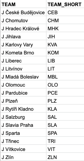
  • =IF(VALUE(MID(F2, 2, 1))=VALUE(MID(F2, 4, 1)), "EV", IF(VALUE(MID(F2, 2, 1))>VALUE(MID(F2, 4, 1)), "PP", IF(VALUE(MID(F2, 2, 1)) We’ll use this tab in the below sections. The Schedule tab As mentioned above, we need to grab the three-letter team name for each team on the schedule. We can again use VLOOKUP here. With the home team in column B and the away team in column C:
    • HOME_SHORT =VLOOKUP(B2, Teams!A:B, 2, FALSE)
    • AWAY_SHORT =VLOOKUP(C2, Teams!A:B, 2, FALSE)

    We’ll use this data in the next section.

    The GP tab

    The GP tab is a full listing of every player who appeared in each game, so it has many more rows than any of the previous tabs. There were a total of 11,703 player games played in the 2019–20 season of the Czech U20 league. We’ll use this tab to calculate a lot of the stats mentioned in the "Goals" section above on a per-game basis, which we’ll then use to calculate season totals.

    • =VALUE(REGEXEXTRACT(F2, "[0–9]+"))

    Since all the team information we have is whether the player was on the home team or the away team, let’s use VLOOKUP to pull the three-letter team name and the opponent’s team name. If the player was on the home team, pull the home team from the Schedule tab. Otherwise, pull the away team:

    • TEAM =IF(B2="H", VLOOKUP(A2, Schedule!A:E, 4, FALSE), VLOOKUP(A2, Schedule!A:E, 5, FALSE))
    • OPP =IF(B2="H", VLOOKUP(A2, Schedule!A:E, 5, FALSE), VLOOKUP(A2, Schedule!A:E, 4, FALSE))
    • SUMIFS(the range you want to sum up, a range you want to test against specified criteria, the criteria you want the range to meet, a second range you want to test against specified criteria, the criteria you want the second range to meet)

    For example, let’s say you want to total up how many apples you sold from a list of all fruits sold, with the item sold in column A and the quantity sold in column B:

    

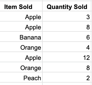
    =SUMIFS(A:A, B:B, "Apple") will get you the total apples sold.

    For each player and each game, we’ll need to calculate how many even-strength goals the player was on the ice for, how many even-strength goals each team scored, and the number of even-strength goals that were scored while the player was not on the ice. We’ll be summarizing data from the Goals tab. The relevant data is in the following ranges:

    • Even-strength goals: column I of the Goals tab has a 1 for each even-strength goal
    • GAME_ID: column A of the Goals tab
    • The scoring team: column C of the Goals tab
    • TEAM_EV_GF =SUMIFS(Goals!I:I, Goals!A:A, A2, Goals!C:C, I2)
    • TEAM_EV_GA =SUMIFS(Goals!I:I, Goals!A:A, A2, Goals!C:C, J2)

    To calculate how many even-strength goals the player was on the ice for, we’ll use the PLUSSES (column S) and MINUSES (column T) columns we set up earlier in the Goals tab. To do this, we’ll use REGEXMATCH to see whether the player’s PLAYER_ID (starting with a P or M and ending with an X) is found in the PLUSSES column or the MINUSES column. REGEXMATCH will return "TRUE" if a match is found, or "FALSE" if a match is not found. However, if we try to use the REGEXMATCH function on our PLUSSES column, we’ll hit an error. To avoid this, we need to wrap our whole formula with ARRAYFORMULA, which allows us to use functions on a range that we would otherwise only be able to use on one cell:

    • PL_EV_GF =ARRAYFORMULA(SUMIFS(Goals!I:I, Goals!A:A, A2, REGEXMATCH(Goals!S:S,"P"&H2&"X"),TRUE))
    • PL_EV_GA =ARRAYFORMULA(SUMIFS(Goals!I:I, Goals!A:A, A2, REGEXMATCH(Goals!T:T,"M"&H2&"X"),TRUE))

    To calculate the number of even-strength goals that were scored for or against a player’s team while the player was not on the ice, we can simply subtract the PL_EV_GX numbers from the TEAM_EV_GX ones.

    Summarizing all of the data

    Creating a list of players

    We now have everything we need to calculate season totals for each player. To do this, let’s create a new tab named Totals.

    • =UNIQUE(GP!H2:H)
    • =UNIQUE()
    • =SORT(data range you want to sort, the number of the column you want to sort by, a TRUE if you want to sort in ascending order or a FALSE if you want to sort in descending order)
    • =SORT(UNIQUE(), 2, TRUE)

    Looking at the player names, we’ll see that the last names are in capital letters and there are a lot of diacritics, or accented letters. For example: David SÝKORA

    • =PROPER(David SÝKORA) = David Sýkora
    • =REGEXREPLACE(David Sýkora, "ý", "y" = David Sykora
    • =REGEXREPLACE(cell containing text, "(ò|ó|ô|õ|ö|ø|ð)", "o")
    • =REGEXREPLACE(REGEXREPLACE(REGEXREPLACE (REGEXREPLACE(REGEXREPLACE(REGEXREPLACE (REGEXREPLACE(REGEXREPLACE(REGEXREPLACE (REGEXREPLACE(REGEXREPLACE(REGEXREPLACE (REGEXREPLACE(REGEXREPLACE(REGEXREPLACE (REGEXREPLACE(REGEXREPLACE(REGEXREPLACE (REGEXREPLACE(REGEXREPLACE(REGEXREPLACE (REGEXREPLACE(REGEXREPLACE(REGEXREPLACE (REGEXREPLACE(REGEXREPLACE(PROPER(B2), "(À|Á|Â|Ã|Ä|Å)", "A"), "(à|á|â|ã|ä|å)", "a"), "(Ò|Ó|Ô|Õ|Õ|Ö|Ø)", "O"), "(ò|ó|ô|õ|ö|ø|ð)", "o"), "(È|É|Ê|Ë)", "E"), "(è|é|ê|ë|ě)", "e"), "(Ç|Č)", "C"), "(ç|č)", "c"), "Ð", "D"), "(Ì|Í|Î|Ï|ì|í|î|ï|i)", "i"), "(Ù|Ú|Û|Ü)", "U"), "(ù|ú|û|ü|ů)", "u"), "Ñ", "N"), "(ň|ñ)", "n"), "Š", "S"), "š", "s"), "Ÿ", "Y"), "ý", "y"), "ř", "r"), "ž", "z"), "Ž", "Z"), "ť", "t"), "Ř", "R"), "Ď", "D"), "ď", "d"), "Ľ", "L")

    Calculating totals

    • =COUNTIF(range you want to check, criteria that needs to be met in order to be counted)
    • =COUNTIF(GP!H:H, A2)

    As mentioned above, SUMIFS can be used for the majority of the other totals. One thing you may notice if you’re copy-pasting formulas from one column to another is that Google Sheets will automatically shift your formula over. So if you’re summing column G in one formula, but then paste that formula one column to the right, Google Sheets will automatically make the new formula sum column H. To avoid this, add dollar signs in front of your cell and range references to lock them when copy-pasting.

    • E: EV_G =SUMIFS(Goals!I:I, Goals!O:O, A2)
    • F: EV_A1 =SUMIFS(Goals!I:I, Goals!P:P, A2)
    • G: EV_A2 =SUMIFS(Goals!I:I, Goals!Q:Q, A2)
    • H: PP_G =SUMIFS(Goals!J:J, Goals!O:O, A2)
    • I: PP_A1 =SUMIFS(Goals!J:J, Goals!P:P, A2)
    • J: PP_A2 =SUMIFS(Goals!J:J, Goals!Q:Q, A2)
    • K: SH_G =SUMIFS(Goals!K:K, Goals!O:O, A2)
    • L: SH_A1 =SUMIFS(Goals!K:K, Goals!P:P, A2)
    • M: SH_A2 =SUMIFS(Goals!K:K, Goals!Q:Q, A2)
    • N: EV_GF =SUMIFS(GP!M:M, GP!H:H, A2)
    • O: EV_GA =SUMIFS(GP!N:N, GP!H:H, A2)
    • P: OFF_EV_GF =SUMIFS(GP!O:O, GP!H:H, A2)
    • Q: OFF_EV_GA =SUMIFS(GP!P:P, GP!H:H, A2)
    • EV_GF% =IFERROR(ROUND(EV_GF/(EV_GF+EV_GA), 4)*100, 0)
    • EV_GF%Rel =IFERROR(ROUND((EV_GF/(EV_GF+EV_GA)-(OFF_EV_GF/(OFF_EV_GF+OFF_EV_GA))), 4)*100, 0)

    We now have one sheet that contains all the summarized stats for each player who played a game during the season:

    

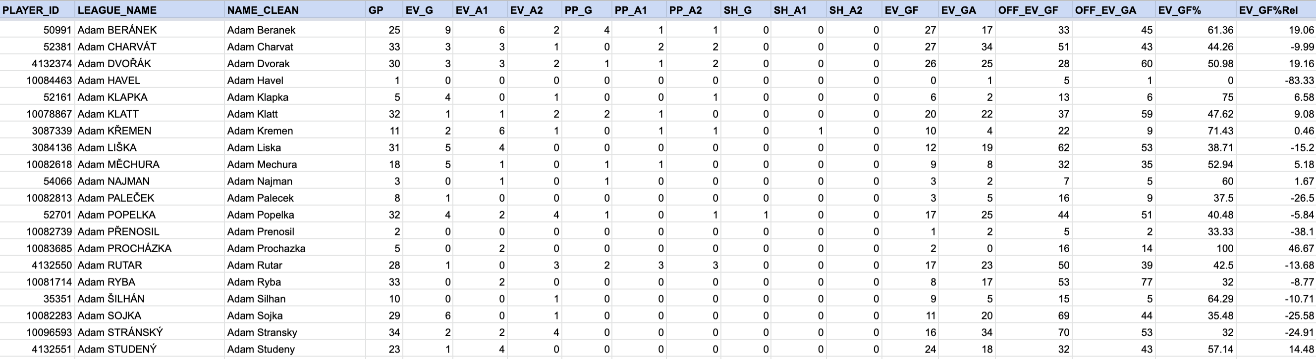
    It’s important to check our numbers, so we can quickly check to make sure total games played equal the 11,702 rows from our GP tab and total goals (EV_G + PP_G + SH_G) equal the 2,150 rows from our Goals tab.

    Summary and next steps

    Throughout the above sections, we’ve taken raw data scraped from the Czech U20 league website and summarized it into season totals for each player, all in Google Sheets.

    Some other steps I take with this data before adding it to Pick224 include scraping the biographical data for each player (birthdays, heights, and shot handedness) and joining that with the summarized data. I also pull each player’s most recent jersey number and the teams they played for during the season. You can find my final results on Pick224.

    As mentioned in the introduction, the first version of the database used for my website was entirely built using the methods above. Once I learned what I wanted to do with my data, I was then able to code a lot of these steps using a programming language, allowing me to run the code much more efficiently. If you would like to make that jump, I suggest you check out Meghan Hall's work on "Moving Beyond Excel for Your Hockey Analysis".

    If data cleaning isn’t for you and you’d rather jump right into analysis, feel free to download any of the data available on Pick224. If you do something cool with the data, please let me know!